9.6 Optimal Triangulation

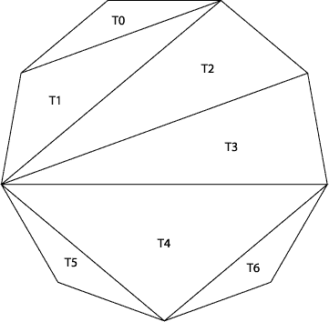
Triangulation - dividing a surface up into a set of triangles - is the first step in the solution of a number of engineering problems: thus finding optimal triangulations is an important problem in itself.

Problem

Any polygon can be divided into triangles. The problem is to find the optimum triangulationi of a convex polygon based on some criterion, eg a triangulation which minimises the perimeters of the component triangles. 

Dynamic programming and optimal triangulation

1. Three seemingly unrelated problems.

Optimal scheduling of matrix multiplications

Matrices (two-dimensional arrays) can be multiplied by the standard formulas from linear algebra: if A*B=C, then C[i,k] = sum A[i,j]*B[j,k]. If A has dimensions x*y, and B has dimensions y*z, then the time for performing these sums in the straightforward way is O(x*y*z). There are more efficient but more complicated matrix multiplication algorithms, but they're not really relevant for today's lecture. Matrix multiplication has many applications including computer graphs and relevance ranking for information retrieval. Now, suppose that you have more than two matrices to multiply. Matrix multiplication obeys the associative law A*(B*C)=(A*B)*C, so there's more than one order in which to do the multiplication. However, the amount of time to do it might be very different. If, say, A is 10*1000, B is 1000*4, and C is 4*200, then multiplying A*(B*C) would take rougly 10*1000*200 + 1000*4*200 operations, while multiplying the other way as (A*B)*C would give the much smaller number 10*1000*4 + 10*4*200. More generally, you could be given a sequence of n matrices M_i to multiply, for i ranging from 1 to n, where the sizes of the matrices are given by a one-dimensional array D: each M_i has dimensions D[i-1]*D[i]. If you could spend a small amount of time planning the optimal order to multiply these matrices, this could lead to a big savings in the time to actually perform these multiplications. However, the number of different multiplication orderings grows exponentially in n, so it would take too long to examine each one and determine its operation count. How can we find the optimal multiplication ordering in an amount of time measured by a slowly growing function of n?

Optimal binary search tree construction

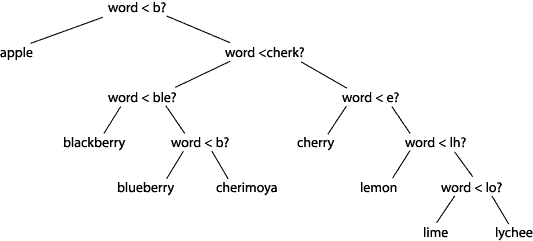
Suppose you have a situation where you will need to match input text against a list of keywords. A standard technique for this is a binary search tree: a tree in which each internal node represents some string comparison, and each leaf represents one of the keywords we are searching for. We perform a search by following down a path in this tree, performing the indicated comparison at each node, until we reach a leaf. To keep things simple for this lecture, I'm going to assume that all comparisons are of type (a < b) or (a < b) rather than allowing equality tests or three-way comparisons, and that we will only search for strings that are already in our list of keywords. Here's a simple example:

The time to search for a given word is just the length of the path from that word to the root; in this example, all words have the same height, and all require three comparisons per search. However, if we have some idea of the frequencies with which we'll encounter each word, we can do better. The average search time would then be sum p(i)*h(i) where p(i) is the frequency or probability of seeing word i and h(i) is its height in the tree. If some words (like apple) have relatively high frequencies, and others (like cherimoya) have low ones, we can reduce the average time by moving the high-frequency words higher in the tree, at the expense of increasing the path lengths for the low-frequency words:

So, if we are given a sequence of words, and the frequencies of each word, how can we come up with an optimal search tree, one that has the minimum possible value of sum p(i)*h(i)?

Optimal triangulation of simple polygons

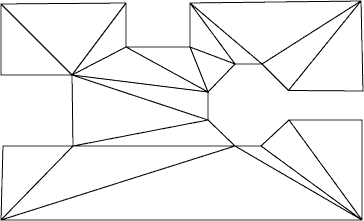
The finite element method is a technique for solving numerical problems such as stress or heat flow simulations, that involves dividing an input shape into simple elements such as triangles, setting up a set of linear equations describing the relations between the simulated quantities in each element, and solving these equations. The solution time and accuracy both depend on the quality of the triangulation: generally, it is desired that the triangles be as close to equilateral as possible.

There has been a lot of work in the finite element mesh generation community on how to measure mesh quality. One commonly used measure for the quality of a single triangle is its area divided by the sum of the squares of its three edge lengths. The goal would then be to find a triangulation in which every triangle has quality greater than some threshhold Q, and in which Q is as large as possible; that is, we are trying to maximize the minimum quality of any triangle. A closely related problem of more theoretical interest is to find the triangulation maximizing the sum of the lengths of all the edges. One of the reasons this is interesting is that, when the input is just a set of vertices and the triangulation must cover their convex hull, we do not know the problem's complexity: we don't have a polynomial time algorithm, nor a proof that it is hard. However, for simple polygons (polygons without holes, in which the triangulation vertices are only allowed to lie on polygon vertices) both of these optimal triangulation problems can be solved by dynamic programming.

2. Abstract formulation

By viewing these problems more abstractly, we can view these problems in a common framework. We take the point of view of the third problem, optimal triangulation, but now we restrict our attention to triangulations of regular polygons. We assume that each possible triangle T in a triangulation has a quality q(T), and that we have a binary operation @ that lets us combine the quality of several triangles. We seek the triangulation of the regular n-gon that minimizes or maximizes q(T0) @ q(T1) @ q(T2) @ ... where T0, T1, T2, etc., denote the triangles in our triangulation.

In order for this to make sense independent of the indexing of the triangles, the binary operation @ should be commutative and associative. In all our examples, @ will be one of the sum, minimum, or maximum operations.

3. Relation of abstraction to initial problems

Optimal triangulation of simple polygons

It is most easy to see how this abstract problem matches the optimal simple polygon triangulation problem. Each vertex of the simple polygon can correspond one-for-one with a vertex of a regular polygon, and this correspondence takes triangulations of the simple polygon to triangulations of the regular polygon. For the case of the max-min-quality triangulation, we can measure the quality of a regular polygon triangle by examining the quality of the corresponding triangle in the input, however if a triangle would be disallowed because it crosses the input polygon's boundary, we give the corresponding regular polygon triangle quality zero. We let @=min and seek to maximize q(T0) @ q(T1) @ q(t2) @ ... which is just the minimum quality of any triangle in triangulation of the input, or zero when the regular polygon triangulation does not correspond to a triangulation of the input. Similarly, to represent the minimum weight triangulation problem, we let q(T) be the perimeter (or +infinity if the regular polygon triangle corresponds to a triangle crossing the boundary of the input polygon), let @=sum, and seek to minimize q(T0) @ q(T1) @ q(t2) @ ..., which is just the perimeter of the input polygon plus twice the weight of the chosen diagonals.

Optimal binary search tree construction

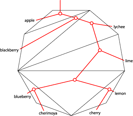
To see how this regular polygon triangulation problem corresponds to construction of optimal binary search trees, draw the search tree words in order around the polygon's sides, except for the top side which will correspond to the tree root. Form a tree by placing a node in each triangle and connecting it across the three sides of the triangle to neighboring nodes or to the words outside the polygon.

Conversely, from any search tree we could reverse this process and form a triangulation. The quality of a search tree is the sum of the frequencies of the words under each node: @=sum, q(T)=sum of frequencies of sides below the top edge of T in the triangulation. To find an optimal binary search tree, we should look for the triangulation minimizing q(T0) @ q(T1) @ q(t2) @ ...

Optimal scheduling of matrix multiplications

To view matrix multiplication ordering as an optimal triangulation problem, label the sides of the regular polygon (except the top) with the matrix names, and the vertices of the polygon with the matrix dimensions. Label each diagonal of a triangulation with the product of the two labels on the triangle below it (below meaning opposite from the top edge).

The top edge will end up labeled with a formula for multiplying all the matrices together. Conversely, from any such formula we can determine a triangulation. To count the number of operations for matrix multiplication, we should simply let @=sum and q(T) be the product of the three numbers written at the corners of each triangle T.

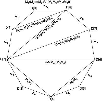
4. Dynamic programming solution

Recall that in any dynamic programming problem we want to identify a set of subproblems to solve with the following properties:

• There is only a small number of distinct subproblems.
• The original problem, and each subproblem, can be solved quickly once we know the values of certain smaller subproblems.

The algorithm works by solving all the subproblems in a systematic order, using an array to store all the subproblem values. For these optimal triangulation problems, we define a subproblem to be the optimal triangulation of the smaller polygon lying below one of the diagonals of the original polygon. A subproblem can be indexed by a pair of numbers: the positions of the vertices on either end of the diagonal (these are the same numbers we used to index array D in the matrix multiplication problem). Each subproblem can be solved by trying all possibilities for its top triangle, using the precomputed values of the smaller subproblems on either side of the top triangle.
In the pseudocode below, the subproblem values are stored in an array V[i,j]. The quality of a triangle is measured by a function q(i,j,k), where i, j, and k are the positions of the three triangle corners. We assume we are trying to minimize q(T0) @ q(T1) @ q(t2) @ ... as in most of the applications above; it is trivial to modify the code to maximize it instead (as in the mesh generation application). We use Python syntax, with minor modifications such as the use of the @ operation and a more intuitive syntax for loops over integers ("for x < i < y" means that i takes on all integer values that make the comparisons true). The constant "id" denotes the identify element for the @ operation: zero if @ is addition, -infinity if @ is maximization.

for n > i >= 0:
    for i < j <= n:
        if i == j-1:
            V[i,j] = id
        else:
            V[i,j] = min([q(i,k,j) @ V[i,j] @ V[j,k] for i < k < j])

The last line of the pseudocode constructs a list of j-i-1 values and finds the minimum value in the list. Here it is again with that line expanded out into a loop of constant-time operations:

for n > i >= 0:
    for i < j <= n:
        if i == j-1:
            V[i,j] = id
        else:
            V[i,j] = infinity
            for i < k < j:
                V[i,j] = min(V[i,j], q(i,k,j) @ V[i,k] @ V[k,j])

As a student pointed out in class, the outer loop needs to run backwards so that all the smaller V[x,y] values will be available when needed. Since the algorithm consists of three nested loops, each of which iterates at most n times, the total time is O(n³). As in the longest common subsequence problem, this code merely computes the value of the optimal solution; to find the solution itself involves a simple linear-time backtracking procedure through the computed array values.